임계값 이동이 필요한 이유
분류모델에서 임계값을 이동하는 경우는 데이터셋의 클래스가 불균형할 때이다.
클래스가 더 많은 쪽으로 임계값을 이동하여, 클래스 불균형을 해소하고 예측 성능을 높일 수 있다.
( 임계값은 0.5가 default 값이다.)
분류 모델 평가지표에 대한 설명은 다음 포스팅을 참고(https://datapilots.tistory.com/41)
타이타닉 데이터로 임계값 설정에 따른 평가지표 & ROC 곡선의 변화를 살펴보자.
0. 라이브러리 임포트 & 데이터 불러오기
import pandas as pd
import numpy as np
import matplotlib.pyplot as plt
import seaborn as sns
from sklearn.model_selection import train_test_split
from sklearn.linear_model import LogisticRegression
from sklearn.metrics import confusion_matrix, accuracy_score, precision_score, recall_score, f1_score
df = sns.load_dataset('titanic')
df_sp=df[['survived','pclass','age','sibsp','parch','fare']]
df_sp.dropna(inplace=True) # 전처리 과정 생략 - 임의로 제거
1. 모델 적용
- 평가지표 함수
#평가지표 함수
def get_clf_eval(y_test, pred):
    confusion = confusion_matrix(y_test, pred)
    accuracy = accuracy_score(y_test, pred)
    precision = precision_score(y_test, pred)
    recall = recall_score(y_test, pred)
    f1 = f1_score(y_test, pred)
    print('오차 행렬')
    print(confusion)
print('정확도: {0:.4f}, 정밀도:{1:.4f}, 재현율:{2:.4f}, f1_score:{3:.4f}'.format(accuracy, precision, recall,f1))- 학습/평가 데이터 분리
X_train, X_test, y_train, y_test = train_test_split(df_sp.drop('survived',axis=1), df_sp['survived'], test_size=0.3, random_state=111)
- 모델 적용
lr_clf = LogisticRegression(solver='liblinear') #데이터양이 적은 경우 사용하는 solver
lr_clf.fit(X_train,y_train) # 학습
pred = lr_clf.predict(X_test) # 예측
get_clf_eval(y_test, pred)

#predict proba : 예측한 클래스의 확률
pred_proba = lr_clf.predict_proba(X_test)
pred_proba로 예측한 클래스의 확률을 가져온다.
2. 임계값에 따라 이진 값으로 변환
from sklearn.preprocessing import Binarizer #임계값에 따라 데이터를 이진 값으로 변환하는 클래스
Binarizer를 사용하여 확률값(pred_proba)을 임계값에 따라 0,1로 변환한다.
임계값 설정과 평가지표 변화
tt_threshold = 0.5 # 임계값 설정

pred_proba_1 =pred_proba[:,1].reshape(-1,1)
binarizer_tt=Binarizer(threshold=tt_threshold).fit(pred_proba_1)
tt_pred =binarizer_tt.transform(pred_proba_1)

get_clf_eval(y_test, tt_pred)
임계값 : 0.5

오차 행렬
[[110  25]
 [ 43  37]]
정확도: 0.6837, 정밀도:0.5968, 재현율:0.4625, f1_score:0.5211
-------------------------------------------------------------
임계값 : 0.6

오차 행렬
[[123  12]
 [ 50  30]]
정확도: 0.7116, 정밀도:0.7143, 재현율:0.3750, f1_score:0.4918
-------------------------------------------------------------
임계값 : 0.4

오차 행렬
[[94 41]
 [30 50]]
정확도: 0.6698, 정밀도:0.5495, 재현율:0.6250, f1_score:0.5848
threshold 0.6 - 임계값 0.5로 설정했을 때 보다 - 정확도 증가, 정밀도 증가, 재현율 감소, f1_score 감소
threshold 0.4 - 임계값 0.5 설정했을 때보다 - 정확도 감소, 정밀도 감소, 재현율 증가, f1_score 증가
임계값에 따라 평가지표 변동이 일어나는 이유
1. 정밀도와 재현율
재현율 : 실제 True인 값들 중 모델이 True로 예측한 비율
정밀도(Precision) : True로 예측한 값들 중 실제 True 인 비율
👉 임계값을 높이면 - 모델이 True 라고 예측하는 비율이 낮아짐 > 정밀도 증가, 재현율 감소
👉 임계값을 낮추면 - 모델이 True 라고 예측하는 비율이 높아짐 > 정밀도 감소, 재현율 증가
2. 정확도
임계값 변화에 직접적인 영향을 받지 않음
👉 전체 예측 중에서 올바르게 예측한 비율이기 떄문에, 하지만 클래스 불균형이 있을 경우에는 변동이 생길 수 있음
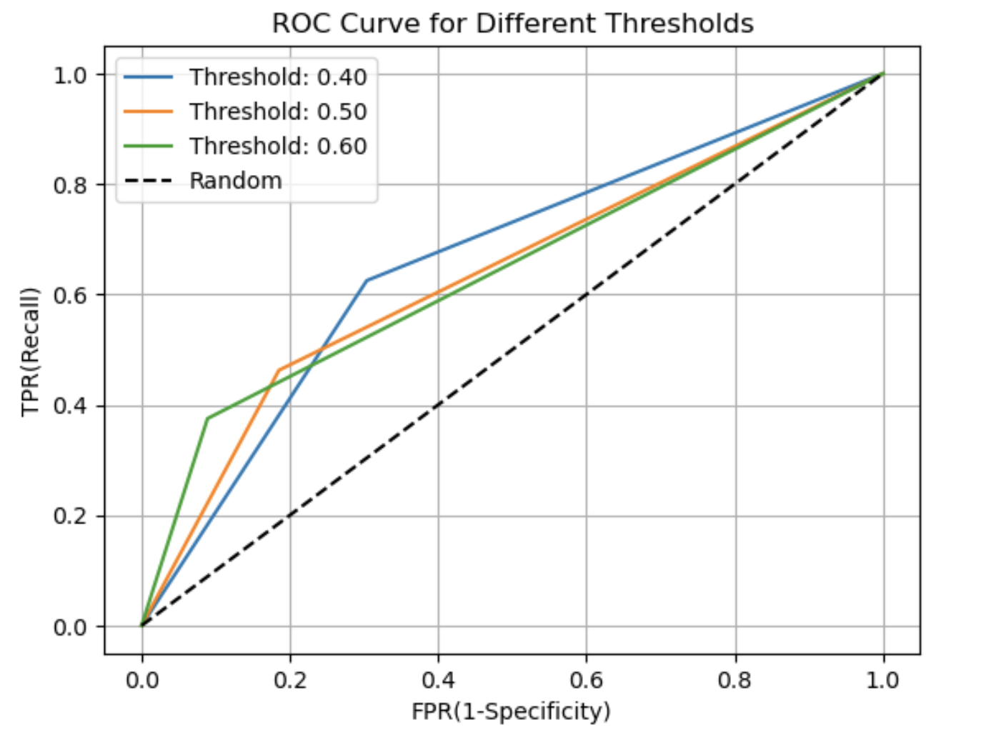
임계값 변화에 따른 ROC 곡선 변화
x축 : TPR (재현율(Recall) : 실제 True인 것들 중 True 예측한 비율))
y축 : FPR( 실제 False 중 True로 예측한 비율)
👉 임계값이 높아지면 재현율이 낮아지고, FPR이 낮아진다 > ROC 곡선이 좌상단에서 우하단으로 이동한다.
import matplotlib.pyplot as plt

def roc_curve_plot_with_threshold(y_test, pred_proba_c1, thresholds):
    for threshold in thresholds:
        # 임계값에 따른 예측 결과 계산
        binarized_predictions = [1 if prob >= threshold else 0 for prob in pred_proba_c1]
        # 임계값에 따른 FPR, TPR 계산
        fpr, tpr, _ = roc_curve(y_test, binarized_predictions)
        # ROC 곡선을 그래프로 그림
        plt.plot(fpr, tpr, label=f'Threshold: {threshold:.2f}')

    # 가운데 대각선 직선 그리기
    plt.plot([0, 1], [0, 1], 'k--', label='Random')
    # 그래프 스타일 설정
    plt.xlabel('FPR(1-Specificity)')
    plt.ylabel('TPR(Recall)')
    plt.title('ROC Curve for Different Thresholds')
    plt.legend()
    plt.grid(True)
    plt.show()

# 임계값 설정
thresholds = [0.4, 0.5, 0.6]
# ROC 곡선 그리기
roc_curve_plot_with_threshold(y_test, pred_proba_class1, thresholds)
'Data Science & AI > Machine Learning' 카테고리의 다른 글
| KNN 알고리즘 모델 적용 - 하이퍼 파라미터(k값, 가중치) (0) | 2024.05.04 |
|---|---|
| [ML]KNN 알고리즘 (2) | 2024.04.07 |
| [ML] 머신러닝 평가지표 - 회귀 모델 MSE, RMSE, MAE (0) | 2023.09.16 |
| [ML] 머신러닝 평가지표 - 분류 모델 평가지표(오차행렬) (0) | 2023.09.15 |
| [Machine Learning] 하이퍼 래퍼 XGBoost API - 위스콘신 유방암 예측 (0) | 2023.08.29 |


